Will it rain today? Will it rain tomorrow? What about at that concert next week or your sister's wedding next year? People intuitively understand weather uncertainty; Sensible quantifies it. Sensible is a weather technology and insurance company powered by cutting edge climate data and research analytics. Sensible understands the needs of quantitatively driven investors and has developed the technology platform necessary to evaluate weather risk for over the counter (OTC) risk transfer markets (aka, "insurance"), as well as exchange- and privately-traded capital and derivatives markets.
Sensible is primarily a weather technology company. Sensible is also a licensed insurance company offering a suite of parametric weather and climate insurance products. The Sensible Weather Insurance Agency, LLC is a nationally licensed insurance producer structured as a managing general agent (MGA) backed by the Sensible Weather Insurance Company - a Bermuda based captive - as well as leading reinsurers operating within the weather risk transfer space. Sensible’s first product line is a consumer-focused set of travel and event insurance policies built to offset experiential losses associated with undesirable weather.
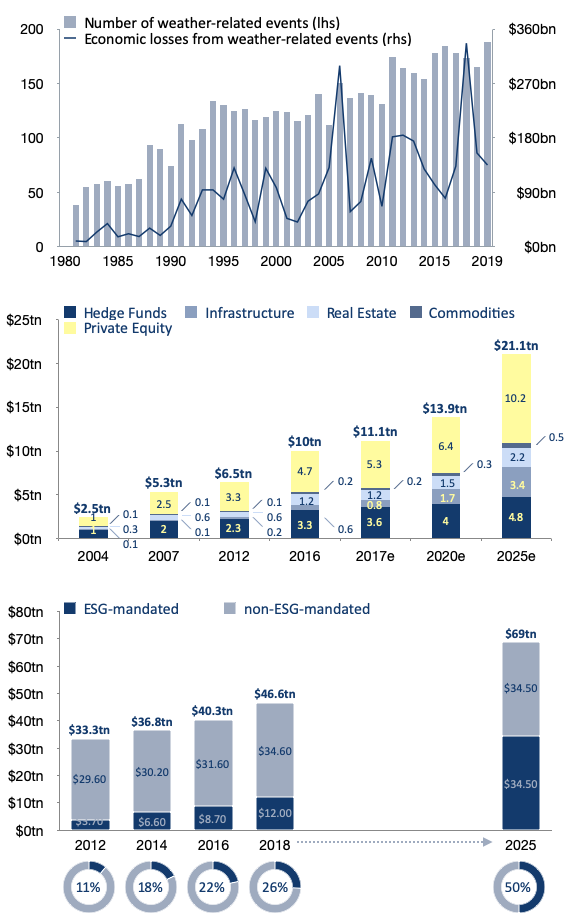
While Sensible’s initial monetization strategy is consumer-focused insurance products, our science-and-technology-first approach has enabled us to create a unique weather technology platform that extends well beyond the scope of parametric insurance alone. Over the past 40 years, the number of economically impactful weather-related events has increased, and so too have the total economic losses arising from these events (Fig. 1, top). The demand for alternative investments - or investments that are uncorrelated with traditional equity and debt markets - increased at a rate of 12.6% per year from 2004 to 2017, and is expected to continue growing at a rate near 8% per year into the future (Fig. 1, middle). The weather-climate system already constitutes a significant opportunity to create an informational edge in some alternative markets (e.g., insurance-linked securities, weather derivatives, certain commodity futures markets), but many more opportunities remain on the horizon. These facts, combined with the increasing demand for environmental, social, and governance related investments (ESG; Fig. 1, bottom), suggest that climate-related finance is primed for explosive growth.
In this document, we outline Sensible’s differentiating features through the lens of a low-order non-linear model built to mimic the behavior of the atmosphere - a tack that we deem to be more approachable than considering a full-blown numerical weather simulation directly. There's a bit of math (!), but we’ll explain the important details in layman terms. We will discuss how the emergent behavior of the model, which readers may find familiar, is analogous to the behavior of the full climate system. Additionally, we draw conclusions about what weather technology is required in order to provide a scientifically consistent probabilistic weather assessment for any time in the future. We conclude with a brief survey of the landscape of the financial opportunities enabled by Sensible’s weather platform.
Are you interested in learning more?
In 1963, Ed Lorenz, a physicist and meteorologist from MIT, published his seminal paper entitled "Deterministic nonperiodic flow" (Lorenz 1963). In this paper, he defined a three variable nonlinear system of equations meant to mimic the behavior of the atmosphere. This model became known as the Lorenz model.
In the Lorenz model, the coefficients σ, ρ, and β represent the physical parameters controlling atmospheric convection, while the x, y, and z coordinates represent the position of an air mass moving through a convective cell. Here, we’ll consider the Lorenz model to be a low order - or "toy" - model of the atmosphere; by design, the emergent behavior of this low order model qualitatively mimics the behavior of full-complexity numerical weather and climate models used in state-of-the-science forecasting and research.
Lorenz painstakingly (computers were much slower then) studied his system of equations using various σ, ρ, and β values combined with various x0, y0, and z0 initial conditions, integrating the system forward with each iteration to study how the system evolves in time. He noted that many, indeed most, combinations of values yielded numerically unstable solutions, or solutions where the x, y, and z values approach positive or negative infinity as time evolves, but that a narrow range of variable coefficients and initial conditions produced a semi-periodic oscillatory-like motion in three dimensions. When integrated for a very long time, the trace of the x, y, and z positions fill out the stable, and hopefully familiar looking, phase space of the dynamical system: the Lorenz attractor (Fig. 2).
The Lorenz attractor is composed of two lobes with a "critical point" at x = 0, y = 0, and z = 0 where no motion occurs. Near this critical point, the system can be described as erratic, where a particle narrowly falls into one lobe or the other as the system moves forward in time. Note that the initial conditions in Figure 2 were chosen intentionally and lie within a very "stable" region of the attractor - when integrating forward in time, it takes a while before the particle gets close to the critical point (i.e., the system is quite "predictable" when starting from this location).
Armed with some knowledge about the way the system behaves, Lorenz then began simulating multiple trajectories simultaneously with the goal of understanding how uncertainty in the initial conditions ultimately impacted the position of a particle at some time in the future - that is to say, he wanted to understand how measurement errors in weather observations might contribute to a lack of predictability in weather models. In Figure 3, we illustrate two particles moving contemporaneously; the first particle is exactly the same as the particle in Figure 2, but the second particle has had its initial conditions ever so slightly perturbed, mimicking the effects of weather observation uncertainty. Put plainly, the first particle represents the actual future, and the second particle represents an error-prone prediction of the future.
In the left panel, we observe the x, y, and z positions of the two particles, and in the right panel, we plot the distance between the two particles as a function of time. We can see that initially, the two particles stay indistinguishably close to each other (i.e., the prediction is good). The two particles remain close to each other until their trajectories near the critical point, at which time they begin to diverge (i.e., the prediction is getting worse). Finally, the two particle’s natural motion leads them into separate lobes, and their trajectories never recover (i.e., the prediction becomes absolute garbage).
Lorenz called the tendency of these two particles to ultimately diverge the "butterfly effect", and used the term "chaos" to describe any such dynamical system which displayed this property.
Chaos - when the present determines the future, but the approximate present does not approximately determine the future.
Finally, Lorenz concludes his absolutely fascinating piece of nearly 60-year old science with the boldest of statements:
"When our results . . . are applied to the atmosphere . . . they indicate that the prediction of the sufficiently distant future is impossible by any method, unless the present conditions are known exactly. In view of the inevitable inaccuracy and incompleteness of weather observations, precise very-long-range forecasting would seem to be non-existent."
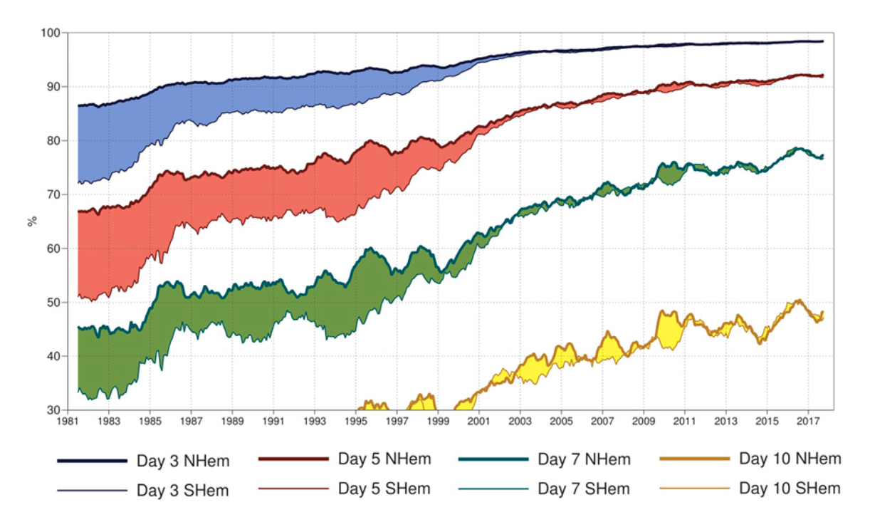
Bear in mind that at this time, the first computational weather model (!), which was run on the first electronic general purpose computer (!!), was barely a decade old. How demoralizing! Of course, it is extremely important to note that since these formative years of modern meteorology and climate research, the science has come a long, long way, and our observations and models are much, much better. But notwithstanding, the skill of weather models is plateauing even despite Moore’s law (Fig. 4); a recent study concluded that a 20% improvement in weather model initial condition uncertainty (a realistic goal for modern remote sensing technology) might only yield improvements in forecast skill of about one day (Zhang et al. 2019).
Historically, the weather forecasting community has focused on combining the most complex weather model with the best estimate of initial conditions, then propagating the system forward in time numerically to produce a single best guess forecast, exactly analogous to what is done in Figure 3. This approach is called "deterministic" forecasting, and rides on the assumption that increasing a model's forecast skill comes down to improving initial condition fidelity alone. But as Lorenz points out, this solution is fraught with challenges and begs the question: is perfection even possible? The philosophical scientist will be reminded of the work of Schrödinger and Heisenberg and the practical scientist might even consider uncertainty in the phase of water molecules at (sub- or super-) saturation! Ghee wiz!
Observing the weather and making sense of those observations is a scientific endeavor in and of itself. One particularly challenging aspect relates to the fact that traditional weather observations, for example from a weather station, are taken at a single point in space and time; even if the sensor is perfectly calibrated, it will only be making precise measurements at one unique location. The weather at any other location may be similar, but will not be exactly the same. For example, it is common for the closest high-quality weather station to be found at the nearest airport, which may be both far away and be representative of a very different microclimate (e.g., that of a large concrete runway) from the actual point of interest. Compounding this issue are various types of measurement uncertainty and bias from the instrumentation itself, human error, reporting error... the list goes on. To combat these issues, weather observations are often averaged and cast into geographic latitude/longitude boxes, forming a mesh or grid over Earth's surface. Gridded data benefits by averaging a large number of independent observations, thereby reducing noise and uncertainty by the law of large numbers, but at the cost of no longer being a true representation of any point within the gridded data's domain. Eliminating initial condition uncertainty entirely would require complete sets of instantaneous observations down to the molecular level, everywhere on Earth. A seemingly impossible feat.
The route forward requires a new perspective; one that embraces chaos and uncertainty. "Probabilistic" forecasting presupposes uncertainty in all facets of modeling: initial conditions certainly, but also boundary conditions and model physics (e.g., do we know σ, β, and ρ exactly?).
In weather and climate science, the most common form of a probabilistic forecast is derived from an "ensemble" forecast. In ensemble forecasting, we embrace that initial conditions are uncertain and that our best guess comes with a substantial margin of error which will, ultimately, materially reduce the skill of a deterministic forecast. So, instead of a single deterministic forecast, multiple sets of initial conditions are created by artificially adding noise to the best guess initial conditions, and from them multiple forecasts are produced, each representing an alternate version of the future. These hypothetical futures can then be considered together to represent the likelihood of a particular outcome.
In Figure 5, we build on top of our Lorenz experiment by adding an ensemble of 500 additional particles, each of which has had its initial conditions randomly perturbed. In the left panel, we can now see the evolution of the true particle, the deterministic particle (whose initial conditions were only slightly perturbed), as well as the 500 ensemble members (whose initial conditions were perturbed even more). In the right panel, we now additionally plot the difference between the average position of the 500 ensemble particles and the true particle. What we see is that, in the near term, the deterministic particle has more skill, however at some point (around t = 1500), the ensemble begins to show more skill, on average, than the deterministic forecast.
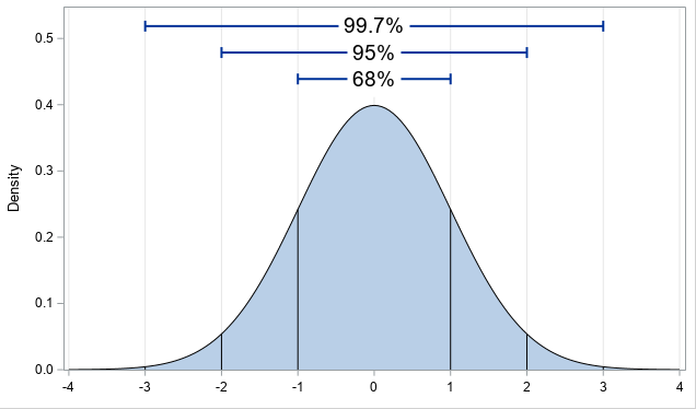
So, as a mid-argument conclusion, we can see that the average, or in statistics jargon the expected value, of the randomly perturbed ensemble tends to have more skill in the long term than the single deterministic forecast. But why stop there? The expected value is just one summary statistic of a "probability density function", or pdf. A pdf succinctly summarizes the probability space of a random variable - for example, the roll of a die has a uniform density distribution where each number, 1-6, is equally likely. The Gaussian, or normal, distribution, shown in Figure 6, is one of the most common and recognizable distributions. The normal distribution is completely described by the mean (aka, the expected value) and the standard deviation, which dictates the width of the pdf. Beyond the mean and standard deviation, the skewness, equal to zero for the normal distribution, is a measure of its asymmetry, the kurtosis is a measure of the thickness of its tails, and so on. The salient feature of pdfs that will be required for the sake of our argument, however, is that regions of higher density equate to regions of higher likelihoods.
In Figure 7, we offer a probabilistic view into the same ensemble we looked at in Figure 5, except now, instead of plotting the forecast error of the ensemble mean, we plot the marginal pdf of x, y, and z estimated from the ensemble distribution as a function of time together with the true position. We see that initially, the pdf of the ensemble is very narrow around the true position of the particle - the forecast is fairly certain of the future. As the forecast evolves, however, the pdfs begin to widen, indicating that the forecast is increasingly uncertain about the future. Often times, pdfs even take on a bimodal shape, indicating that the true particle’s position is most likely either here or there, but not likely in between - a good real world example of this phenomenon is a summer thunderstorm; it either doesn't rain at all or it rains a lot, but it never rains only a little bit. As these pdfs evolve, we can also see that, for the most part, the true particle position moves in line with the peak of the forecast distribution, indicating that the true particle generally lies in the region of probability space where the forecast thinks it likely should be - the probabilistic forecast reliably predicts the odds of future outcomes! Moreover, even when the position of the true particle does not coincide with the peak of the distribution, it always lies within the bounds of the distribution, implying that the model always predicts with some likelihood, however small or large, that the true outcome can happen. Bringing the argument back to reality for one second, this distinction implies that the pertinent question is not will it rain tomorrow?, but rather what is the chance that it rains tomorrow?, and the relevant explanation of what ends up occurring relative to the forecast is not whether the forecast was right or wrong, but rather whether the outcome was or was not likely. The further out the ensemble forecast runs, the more dispersed within the attractor the particles become, and the less "skill" the forecast has in predicting the position of the true particle.
Toward the end of the video, the shape of the pdfs begin to converge. In Figure 8, we start from where Figure 7 leaves off. Now, instead of plotting the evolution of the pdfs in the right panels, we plot the new ensemble pdfs on top of the pdfs from the previous time steps in light blue. Superimposed on top of the ensemble pdfs are the pdfs derived from a very long simulation of a single particle in black. The real-world analogue of this very long simulation is simply a set of actual weather observations from the historical record, which scientists refer to as a climatology. What we observe is that as time progresses, the ensemble forecast pdfs converge on those of climatology, suggesting that the best probabilistic forecast is simply the pdf derived from historical data. In other words, at some point, we are just as well off determining weather odds from historical data as we are from a probabilistic weather forecast (!).
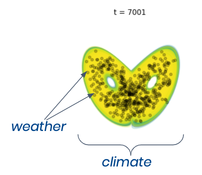
"Climate" is often defined as the long term average of "weather", but as we’ve just observed, an average is actually just the simplest descriptor of the set of weather outcomes which together define the climate. Rather, from our experiments here with a toy weather model, we can now understand the true relationship between weather and climate - a seamless transition from signal to noise quantified through probability (Fig. 9).
Even a topic as important and complex as climate change is not beyond the scope of understanding with our trusty Lorenz model! But before talking about climate change specifically, it is first instructive to consider uncertainty in the Lorenz model parameters, that is σ, β, and ρ, while still talking about weather forecasting (we hinted at this in the first paragraph of Section 2).
State-of-the-science numerical weather prediction models are incomplete mathematical approximations of our atmosphere. For example, due to the inherent computational complexity of producing a weather forecast, most weather models are only able to directly simulate atmospheric physics down to the single digit kilometer scale, meaning that the explicit simulation of smaller scale features (individual clouds, for example) is currently impossible in any operational sense; the behavior of clouds in weather models is most often a statistical approximation. Other types of physics are left out of the models entirely; for example, particulates and aerosols in the atmosphere can have a significant impact on solar transmission - consider Los Angeles on a hazy or smoggy day - but atmospheric chemistry is also generally missing from operational forecasts. On August 21, 2017, NOAA’s same day temperature forecast for New York City missed by over 10F because models failed to account for the precisely predictable passage of the moon in front of the sun - a solar eclipse. Someone probably should have thought of that one.
In the toy Lorenz model, missing or approximated physics is analogous to uncertainty or errors in the Lorenz model parameters σ, β, and ρ. If the errors are small, then in the near term they might not matter, but over time the impact of the model deficiencies accumulate, leading to systematically poor forecasts. As an illustration, in Figure 10, we build on top of our simulation from Figures 7 and 8 by adding a second 500-member ensemble, except that this ensemble has had its parameters altered by an arbitrarily small amount. As we run the forecasts forward, we can see that initially the probabilistic forecast of the biased ensemble closely resembles that of the unbiased ensemble, but that over time the forecasts diverge from each other. Ultimately, the biased forecast will not only lose skill faster than the unbiased forecast, but its skill will turn negative.
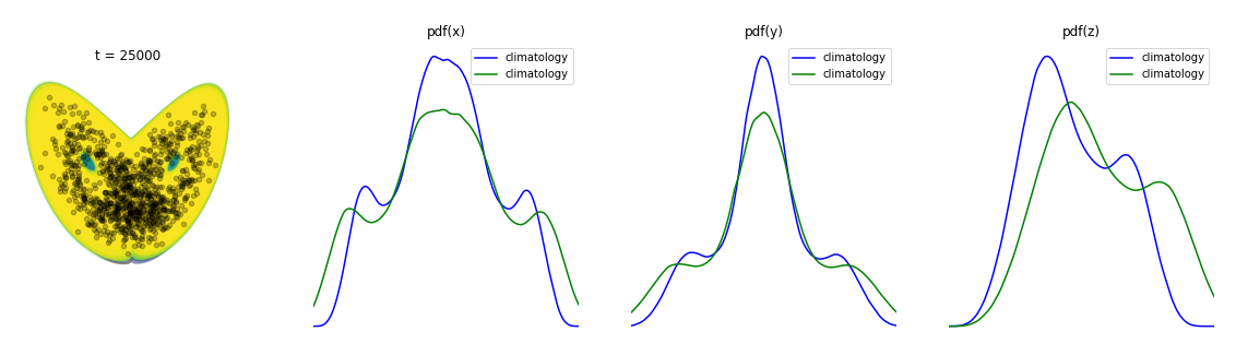
Shifting topics to the question of climate change: the analogy in our toy model world would be if we were to systematically change the Lorenz model parameters σ, β, and ρ as a function of time - this is like saying the normal rules of the game are slowly changing. In Figure 11, we’ve run the simulation in figure 10 out for an arbitrarily long time. We then plot the climatological pdfs of the two simulations on top of each other, and examine the differences. For variables x and y, we can see that the distributions remain symmetric and centered around the same mean, but that the shape of the distributions have changed slightly - from these changes, we would expect that the probabilities of certain x and y events will have changed, but that overall their climates are similar. For variable z, however, we can see that not only has the shape of the pdf changed, it’s also shifted to the right - the future climatology of variable z has certainly changed, and importantly, higher values are more likely. This is quite similar to what we expect for temperature in many locations around the world under future climate scenarios. While climate scientists often report key and digestible warnings like a change in global average temperature of roughly 9℉ by the year 2100, the reality is entire pdfs of temperature are changing in predictable ways and that those changes will vary from place to place.
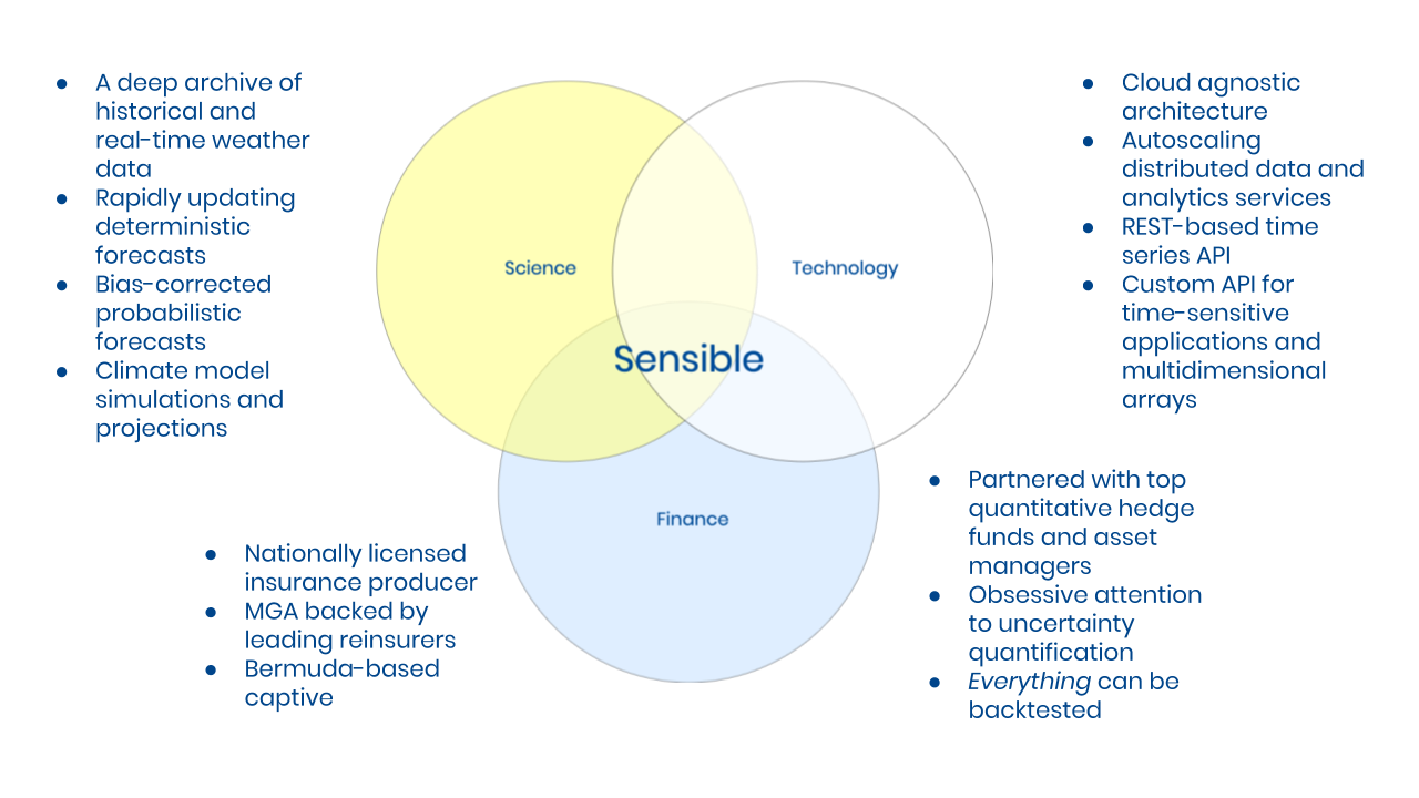
Sensible uses the principles described in the previous sections to power a weather technology platform built specifically for financial trading and risk transfer applications. Our system is designed to house both gridded data and point data at global scale and at (sub-) hourly resolutions. Our weather data is composed of
- A deep archive of historical and real-time weather observations;
- Rapidly updating deterministic forecasts;
- Bias-corrected probabilistic forecasts;
- Climate model simulations and projections.
These data sources allow us to build analytical models using historical data sources while mapping these models onto probabilistic forecasts for any time horizon. Our proprietary technology stack is composed of
- A cloud agnostic architecture;
- Autoscaling distributed data and analytics services;
- REST-based time series APIs;
- Custom APIs for time-sensitive applications and multidimensional arrays.
Our data pipelines are designed to be parallelized and to operate in a distributed cloud environment, allowing us to fulfill data requests and analytics in a scalable way, all in real-time. Additionally, multiple layers of usage data are used to construct optimization feedback loops, which, together with multiple levels of caching, enables our system to become more efficient as it scales.
The key to developing and maintaining Sensible’s powerful technology stack and sizeable data processing technology stack relies on the fact that our monetization scheme is based on enabling financial risk taking, rather than packaging and selling weather data alone. The Sensible founding team has decades worth of collective experience at the intersection of weather and finance, specifically with a focus on insurance and insurance-like products. In addition to being a weather technology platform, Sensible is a
- Nationally licensed insurance producer
- MGA backed by leading reinsurers
- Bermuda-based captive
focused on offering scalable parametric insurance products. Sensible also partners with selected quantitative hedge funds and asset managers, providing them with unparalleled data access and weather risk management tools which, in addition to being product-complete, have been built with obsessive attention given to uncertainty quantification and backtest capabilities.
Sensible believes that weather as an asset class is just showing the tip of an iceberg. According to the US Department of Commerce, $4T of US annual GDP is impacted by the weather. Catalyzed by increasing climate risk exposure, accelerating climate change, and a growing pool of capital earmarked for alternative risk and ESG investments, an increasing number of climate related financial opportunities will arise in the years to come.
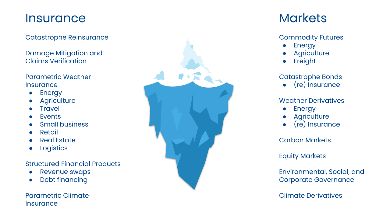
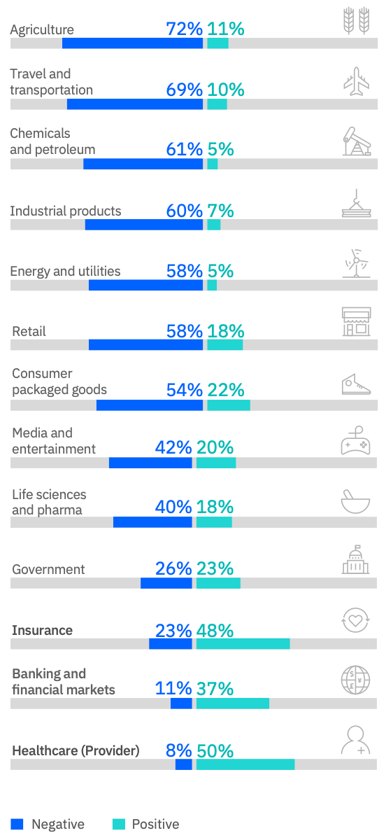
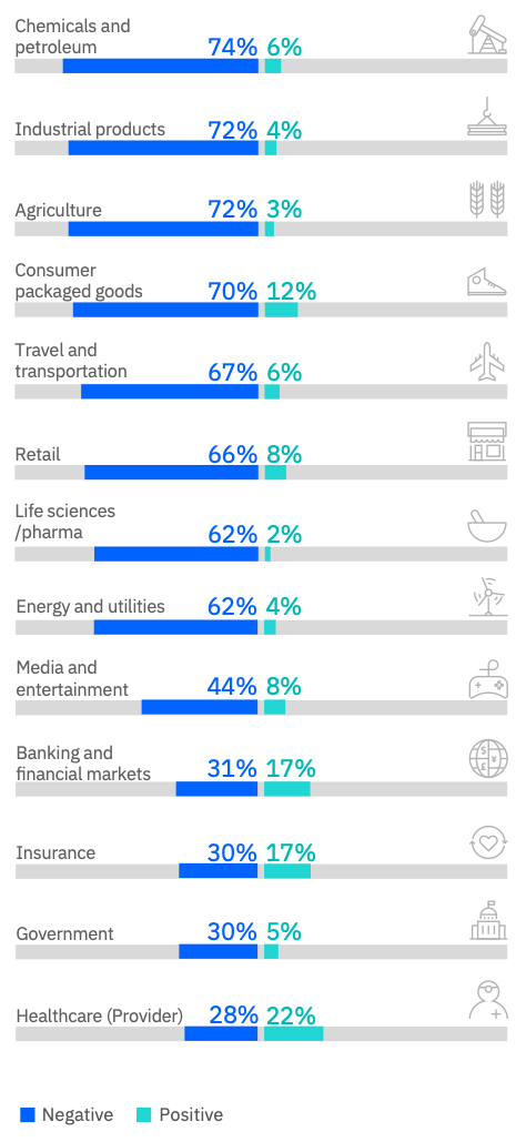
Economic weather impacts can be succinctly summarized by examining impacts on cost and revenue separated by industry. Historically, insurance- and market-based solutions have been employed in agriculture and energy to manage weather risk, but many other industry sectors can have either their revenues and/or costs be weather impacted as well (Figs. 15, 16).
Sensible has chosen the consumer-facing travel and events sectors to focus on first. Through these markets, Sensible's goal is to achieve the widest possible product education and distribution, thereby distancing itself from its competitors through technological superiority and brand recognition. Wide distribution, paired with a naturally diversified portfolio of episodic travel- and events-related weather risks, will enable increased access to the efficient capital necessary to unlock the remaining weather impacted industries.
References
[1] Deloitte. (2020). Advancing environmental, social, and governance investing.
[2] IBM Institute for Business Value. (2018). Just add weather: How weather insights can grow your bottom line. 22pp.
[3] Lorenz, E. N. (1963). Deterministic Nonperiodic Flow. Journal of the Atmospheric Sciences. 20 (2) 130-141.
[4] pwc. (2018). Rediscovering alternative assets in changing times. 18pp.
[5] SwissRe. (2020). sigma: Natural catastrophes in times of economic accumulation and climate change. No 2.32pp.
[6] Zhang, F., Sun, Qiang Sun, Y., Magnussun, L., Buizza, R., Lin, S-J., Chen, J-H., Emanuel, K. (2019). What is the predictability limit of midlati- tude weather?. Journal of the Atmospheric Sciences. 76. 1077-1091.